InStep - Help

Decimation Tool - Options

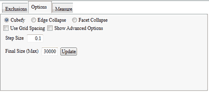
Options Tab

The options available will depend on the algorithm selected. The default algorithm is the Cubefy algorithm which is a very fast and robust approach but does not guaranteed a solid body. The approach relies on shifting each vertex to a grid that is coarser than the original data, essentially rounding the location's components. By doing so, the vertices will - once the grid is sufficiently coarse - form degenerate facets (where two or more vertices are the same) and thus no longer be required. The algorithm allows for two different methods to reach the target: by Grid Spacing or by Final Size (default). The grid spacing approach is a direct approach that utilizes the user supplied grid size (Grid Spacing) to define the rounded step size of the components (in the work units). By setting a larger spacing, more facets become collapsed and thus the final size is smaller.
Alternatively, the algorithm can determine the best grid spacing iteratively (Use Grid Spacing is unchecked). This approach is the same as the grid spacing approach but iterates until the Final Size has been met or exceeded. The Step Size in this case is the incremental size by which the overall grid is to be coarsened. In some cases this step size can be quite small, in other cases it should be quite large and depends on the model size, feature size and applicable units. It is recommended that, for large files, the single step approach is first used to estimate what the outcome is rather than to have an incorrect starting size and then spend a long time iterating.
The Advanced options allow the algorithm to be further modified. If the grid is not to be scaled uniformly, non-uniform sizing can be applied to the X,Y and Z direction. The Smooth Perimeter option adds an additional set of facets around those already selected in the exclusions tab and then moves them according to the adjoining normal vector and a user defined multiplier. In some cases it may also be necessary to constrain the change of the coordinate components along only one or two axes. In this case the X,Y,Z Axis can be prevented from being moved.
Once the algorithm completes, the overall shape is usually quite coarse (it has been cube-fied), by Re-Applying the locations, the body becomes smooth again. The options are to either use an original location (useful in cases where specific locations are to be used for later tracing or regeneration in a CAD application) or an Average location defined by all the vertices that have become collapsed to the new location.

The Edge Collapse algorithm, as its name implies, works by selectively collapsing edges and thereby reducing the number of facets by two (usually) per iteration. Unlike the Cubefy algorithm, this approach allows a metric to be defined by which an edge is to be collapsed or kept. Aside from the exclusion selection, this algorithm uses a cost based selection which removes a set of facets if their overall contribution to the model is small. Since it is an iterative approach, it is slower than the Cubefy option though still reasonably fast for large bodies (in the order of a few 100,000 facets). Since it is iterative, it also reaches the target size more accurately (usually within one or two facets of the required size). Only a few options are available for modification of this algorithm: Edge Length and Vertex Angle Power. Both these values define how much relative importance is to be put on the length of an edge (remove smaller ones first) vs. removing items that have a small angle between facets (items that are parallel should be removed first since they do not add additional information to the overall body). Use of either parameters should only be done after first evaluating the default values and should only be done in a small range of values (0.5-2.0 is recommended).

Additionally, the Edge Collapse also has the option to collapse 'By Cost'. This offers the ability to reduce the data until either the target number of facets has been reached (determined by the 'Final Size' entry) or until the cost value of the next collapse is larger than the allowable value. 'Cost' in this case is somewhat difficult to quantify but represents a value that is equivalent to the differences in angle (in radian) between the original and potentially new configuration multiplied by the length of the edge that will be collapsed. The value does not carry any significant units (radian-meter essentially) and will need to be used on a trial and error basis. What this can be successfully used for however is to collapse 3D scan data where facets may have been used that are almost flat on a surface (so slightly 'bumpy' due to inaccuracies in the scan) and thus collapsing several may have a cost that is very small, usually around 0.1 to 0.01. By first collapsing all items that have a value smaller than (for example) 0.1 and then examining the resultant data, a high level of detail can be maintained by only collapsing items that are essentially flat or negligible.

The Facet Collapse algorithm is similar to the Edge Collapse but works on the entire facet rather than edges only. Since collapsing a single facet can affect three (or more) facets, it is considered less robust than the edge collapse approach but does have some benefits. In addition to the items discussed for the edge collapse approach, the facet collapse allows facets to either be collapsed to their center point or to the Least-Change vertex, meaning that the original vertices of a facet are checked for what causes the least amount of change in the overall body and this facet is then used as the target for the others move. Since this option requires an iterative operation, it does slow down the process but can yield better results. Additionally, with this approach an option is provided that can ignore the exclusion selection if the target size has not been met once all the other items have been accounted for. Use of this option is not recommended at this point unless the data has been verified.